- Get link
- X
- Other Apps
To analyze data in Excel, you don't need to be an expert in Excel. You just need to know a few functions and tools to get the job done. Compare with financial analysts, they are very expert in excel and they create financial models and staff. They need to know all the shortcuts, functions, designs, layouts and many of them can work in Excel without touching the mouse. But you don't have to be that level of expert to analyze data with Excel.
Before you start working with Excel, first see how many different versions of Excel are available. There are different versions of Excel but Excel 2007(Windows), 2008(MAC), 2010(Windows), 2011 (MAC), Excel 2016, Excel 2019, and Excel 365 are the most popular. Excel 365 is advanced but you can use any version.
Let's start with Excel…
Excel Layout:
First we need to understand Excel layout. At the very top of Excel, that section is called the "Quick Access Toolbar." By default, that section has three menus Save (Ctrl S), Undo (Ctrl Z), Redo (Ctrl Y). However, you can modify as you need.
Then, the section immediately below is called the "ribbon". This section contains File, Home, Insert, Page Layout, Formulas, Data, Review, View, Developer, Help, Power Pivot, Tell Me (Alt Q).

Below the ribbon, there are "Name Box" and "Formula Bar". You can use this formula bar to compose Excel formulas.
Underneath, there is a large blank space where you will do all the calculations. It is called "Sheet". You can create multiple sheets (eg sheet 1, sheet 2, sheet 3, sheet 4….). Together they are called "workbooks".

File format:
Excel has several file formats. Here is the main one listed:
.xls - This is the older file format that Excel uses and you may encounter if you are pulling data from an older system. Always convert data to the new format because their legacy code has many security flaws that Microsoft is under no obligation to fix.
.xlsx – This is the current version of the Excel file format that supports almost all current Excel functions.
.xlsm – This is similar to .xlsx, except it supports macros. Macros are a way you can manage specific functions.
.csv stands for "comma separated values" and is a standard method for sorting data.
Excel data types:
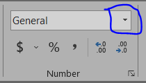
Normal: Normal is a default data type in Excel. It usually takes all kinds of data. It actually predicts the data like if you enter the date it will predict the data as date/custom. The string goes to the left side of the cell and the number goes to the right side of the cell under normal data type.

number: Converts number data type data to numbers. By default, it keeps 2 decimals but you can always change by clicking Decimal Increase and Decimal Decrement.

Number data types have three categories:
· Percentage
· Fractions
· Scientific
Note: If you want to put 0 in front, use it (') in front of the number
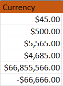
Currency: This will convert any number of data into specified currency

Accounting: Accounting is similar to currency but with some differences. If you convert the number to accounting then automatically align the Dollar sign left. And the negative sign is converted to parentheses. Compare the two data types below for better understanding.

Date Time: Of all data types, the date-time data type poses problems. Use international format 2022-02-27 for date-times. You can easily figure out if the format is like this. Start with the year, followed by the month and then the date. To convert the data type to that format, go to the Number section then click on "More Number Formats".


Time: It converts a date into a time format. Go to time click on "number section" then it will be converted to date.

There are several other data types available such as text, special. Text Converts all data types to text/string and special secret numbers like zip code, social security number to special format.
Aggregation function:
The merge function is applied across a range of cells and summarizes their values into a single cell. There are many different aggregation functions, listed below are some of the most common.
The sum

average
An aggregation function that outputs the average of all its inputs. Like the SUM function, works well with numbers and formats that can be converted to numbers, such as dates

COUNT
A sum function that counts the number of non-zero cells among its inputs. Works with any data format because it only calculates for cell content.

the median
An aggregate function that outputs the median of all its inputs. Like the SUM function, works well with numbers and formats that can be converted to numbers, such as dates

mode
An aggregation function that outputs the most common value of its inputs. Like the SUM function, works well with numbers and formats that can be converted to numbers, such as dates This function works with Excel 2007 and earlier.

MODE.SNGL
This is the modern form of the MODE function and returns only one value like the MODE function.

MODE.MULT
It outputs an array of values for each value that can be considered the mode of the dataset.

MAX/MIN
MAX and MIN are integration functions that determine the largest or smallest value of their inputs. Like the SUM function, works well with numbers and formats that can be converted to numbers, such as dates

Lookups
Lookups allow you to match values from a range to another reference
VLOOKUP
VLOOKUPs are the most common type of lookup and can be used to match data from one range to another. The parameters of a VLOOKUP are as follows.
Worth watching
To see your desired values
table_array
The range from which we want to pull the value. Make sure your lookup value is in the left-most column of the range
col_index_num
The number of columns for the value you want to fetch. 1 refers to the left-most column of your range
range_lookup
Should VLOOKUP find an approximate match or an exact match? This is true by default but you'll usually want an exact match and so set it to false

HLOOKUP
HLOOKUPs are basically the same thing except they work horizontally.
XLOOKUP
This is a new version of the VLOOKUP/HLOOKUP formula. Depending on your version of Excel, you may not have access to this function.
XLOOKUP is a much more flexible version of VLOOKUP and HLOOKUP because it doesn't require your lookup array (the list of matching values) to the left of your return array (the list of values you input).
Worth watching
The value you want to see
lookup_array
List of values that the value you are trying to match can contain
return_array
List of values (same length as lookup_array) from which you are trying to return values
[if_not_found]
A default value to return if you don't find a match between your lookup_value and your lookup_array.
[match_mode]
Excel should try and find an exact match or settle for an approximate one. Unlike VLOOKUP and HLOOKUP, it defaults to an exact match which is what we usually want anyway.
There is also an option for a wildcard match which can be useful if your lookup_value cell doesn't have full information (eg having only the last name instead of the full name).
[search_mode]
Excel should search lookup_array in order
INDEX MATCH... MATCH
The INDEX and MATCH functions, when combined, are very powerful and are used in many advanced Excel functions. It is considered by advanced Excel users a better practice to use VLOOKUP instead if you can. Let's first see what the individual functions do.
INDEX will return any value in a 2D array based on a specified row_num and column_num. Note in Excel that row numbers and column numbers start with 0, not 1.
MATCH will return the index number of a specified value within an array. It can only search 1D arrays so you need to use two match functions to find an item in a 2D array.
You can group two MATCH statements together in the row_num and column_num parameters of the INDEX function:
- =INDEX(B4:F7,MATCH(I7,A4:A7,0), MATCH(H7,B3:F3,0))
IF
One of the most powerful and used functions in Excel. IF allows you to set a condition and then output one value if that condition is met and another if it is not.
There's a common joke among developers that coding is basically a bunch of loops and if statements. With this function, you can replicate some of the functionality of an entire programming language.
logic test
It is conditional that you can assign. Typically, you'll look for a value to be equal to, greater than, or less than another value.
[value_if_true]
This is what Excel should output if the conditions you specified are met
[value_if_false]
Excel should output this value if the condition you specified is not met
Let's say you want to have multiple conditions, this is where Excel's IF statements can get a little tricky. What you want to do is use the AND operator inside the IF function:
- =IF(AND(A2>=3, A2<=5), ">=3 AND <= 5", "None")
SUMIF(S)

COUNTIF

String Functions
CONCAT
CONCAT will take multiple text formatted cells and combine them. You can also input your own text strings inside the CONCAT function to dynamically generate labels.

LEN
The output is the character length of its inputs.

TRIM
Trim any white space at the end of any string you have. This can be especially useful when you're importing CSVs into your workbook because some CSVs are poorly formatted and have trailing or leading spaces in their headers.
Import of multiple CSVs with extra spaces in headers

Formatting
One of the biggest use cases I have for Excel is presenting data from ad hoc analysis where creating a dashboard can be too much of a lift. Typically, I'll pull data using SQL queries and then copy it to Excel to share. In this case, I've found that formatting your outputs correctly can yield huge results and make your stakeholders much happier with your work.
Merge Cells

Center Across Selection

Remove gridlines

Grouping / Ungrouping Cells

Adding and Removing Decimals

Data Validation

Conditional Formatting

Data Manipulation
Properly Importing CSVs

Remote Duplicates

Text to Columns
Filters

Tables
Pivoting
Pivot tables are one of Excel's most useful features and allow you to pivot and transform data in a variety of ways so you can easily and quickly analyze different cuts of data.

Before pivot:

After Pivot:

Comments
Post a Comment